Kinetic Monte Carlo and the One-Dimensional Chromatin Model
I came to kinetic Monte Carlo while studying how nucleosomes are arranged in budding yeast. Nucleosomes are proteins around which DNA is wrapped in eukaryotic cells (think the “spindle” in a “spool of (DNA) thread”).
Experimental assays of nucleosomes show ordered arrays near boundaries: a nucleosome-free region, a transcription-factor site, or the edge of a gene can act as a landmark, and the average positions of the next few nucleosomes oscillate away from it.
The pattern is striking enough to invite a tempting question: are the nucleosomes individually programmed to those positions, or can much of the order emerge from particles packing against a boundary?
I wrote a small kinetic Monte Carlo framework to explore that question. It has C++ and Java implementations, a little visualization infrastructure, and an early Python model of MNase digestion. It is research code rather than a polished package, but it makes the basic model concrete.
That question has a literature behind it. The classic barrier-nucleosome model proposed that a well-positioned nucleosome at a promoter edge can pack its neighbors into progressively less precise arrays, so the first nucleosome past a nucleosome-free region can be sharply phased without every downstream position being encoded independently. Later work made “sequence versus packing” quantitative, treating nucleosomes as one-dimensional hard objects and separating steric exclusion from intrinsic histone–DNA affinity — an array can be ordered because particles cannot overlap, even when their individual sequence preferences are weak. Morozov and collaborators eventually made the statistical mechanics explicit in a one-dimensional model of nucleosome positioning: hard-core particles in a sequence-dependent potential, solved analytically for point particles and numerically for finite ones. My KMC code is the dynamical cousin of that model. Rather than asking only which configurations have weight, it asks how a system with specified rates moves between them.
The smallest useful model
Start with a one-dimensional lattice representing DNA. A particle occupies a footprint of \(a\) base pairs (147 bp for a canonical nucleosome, though a toy simulation might use 10 or 15 sites). If the left edge of particle \(i\) is \(x_i\), hard-core exclusion says \[x_{i+1} \geq x_i + a.\]
There may be a fixed or periodic boundary, and every position can have an energy \(V(x)\). A sequence-dependent potential might make some DNA easier to bend around a histone, while a transcription-factor site or an NFR can be represented as an obstacle or an unusually costly interval. For a configuration of particles, a simple energy is \[E = \sum_i V(x_i),\]
with statistical weight \(e^{-\beta E}\). Even this austere model produces useful observables: occupancy at each base pair, the distribution of linker lengths, and the pair correlation between neighboring particles.
Put one immobile barrier at the left edge and let identical particles fill the line. The first particle has to sit next to the barrier (unless a gap is energetically preferred); the next particle is constrained by the first, and so on. Averaging many configurations produces alternating peaks and troughs whose amplitude decays with distance. This is statistical positioning. Individual molecules can be imperfectly aligned while the population average looks beautifully phased.
That distinction matters. A peak in an occupancy map is evidence about a distribution, not necessarily a command that every cell obeys.
Hard rods on a line: the Tonks gas
Stripped down—identical hard particles of footprint \(a\) on a line, no external potential—this model is exactly solvable. It is a Tonks gas, the classical one-dimensional gas of impenetrable rods that Lewi Tonks solved in 1936.
The rods cannot pass one another, so they stay in order, and the configuration integral can be done by changing variables from positions to the gaps between neighbors. For \(N\) rods on a segment of length \(L\), \[Q_N(L) = \frac{(L - Na)^N}{N!}, \qquad L \geq Na.\]
That is an ideal gas on a shortened line, with the excluded length \(Na\) simply removed. Differentiating the free energy gives the equation of state \[\beta P = \frac{\rho}{1 - \rho a}, \qquad \rho = N/L,\]
which is van der Waals with the attractive term set to zero: the pressure diverges only at close packing, \(\rho a \to 1\).
Two consequences matter for chromatin. The first is that the gaps between neighbors are exponentially distributed, \[p(s) = \beta P\, e^{-\beta P s},\]
with mean \(1/\rho - a\). Pure hard-core packing predicts that the most common linker is the shortest one. Measured linker distributions in yeast are not exponential—they have a preferred length—and that discrepancy is itself evidence that something beyond exclusion is setting the spacing.
The second is the boundary. In the grand canonical ensemble with fugacity \(z = e^{\beta\mu}\) and partition function \(\Xi(L) = \sum_N z^N Q_N(L)\), inserting a rod at position \(x\) cuts the line into two segments that no longer know about each other. The density of particles whose left edge sits at \(x\) on a segment with hard walls is therefore just a product: \[\rho(x) = z\,\frac{\Xi(x)\,\Xi(L - x - a)}{\Xi(L)}.\]
Evaluated near a wall, this is a damped oscillation: peaks spaced by roughly the mean center-to-center distance \(1/\rho\), with an amplitude that decays exponentially over a correlation length \(\xi\). Statistical positioning falls out of two lines of algebra, with no simulation and no fitting.
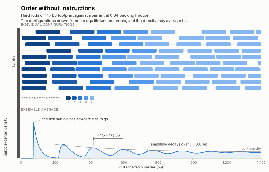
Both panels come from the recursion below rather than from a simulation: the configurations are exact samples from the ensemble, and the curve is the exact density, not a histogram. Nothing in it was fitted. The first particle is pinned—its density at contact is \(\beta P\), six times bulk here—the second is merely constrained by the first, and by the sixth the distribution is nearly flat. Peaks land every 172 bp against a predicted \(1/\rho\) of 175, and the envelope decays with \(\xi \approx 390\) bp. No particle was told where to sit.
It also comes with a built-in limit. The correlation length grows with density, but it is finite for every \(\rho a < 1\), diverging only at close packing—a one-dimensional system with short-ranged interactions has no phase transition and no long-range order. A barrier can phase a handful of neighbors; it cannot phase a chromosome arm. If a map shows an ordered array extending much further than \(\xi\) allows, packing against that barrier is not the whole explanation.
Solving the model without simulating it
Add a sequence-dependent potential \(V(x)\) and the closed form disappears, but exact solvability does not. That is what a companion project, lattice-binding, is for: it computes equilibrium occupancies for the same lattice model directly, without sampling.
The trick is that hard rods on a line still factorize. Walk along the lattice and ask what is at site \(n\): either nothing, or the right end of a particle of type \(g\) with footprint \(m_g\). That gives a recursion for the grand partition function of the first \(n\) sites, \[\Xi(n) = \Xi(n-1) + \sum_g z_g\, e^{-\beta V_g(n - m_g + 1)}\, \Xi(n - m_g),\]
and the same recursion run backward from the far end gives \(\Xi^{R}(n)\). The probability that a particle of type \(g\) occupies the interval starting at \(i\) is then a forward term times a backward term times its own Boltzmann weight, divided by \(\Xi(L)\). One sweep in each direction yields exact occupancies at every base pair, in \(O(L)\), for an arbitrary landscape.
The repository implements that recursion (the “DynaPro” solver) alongside a transfer-matrix solver, which assembles the same object as a sparse matrix product and can also carry two-body interactions between neighboring particles; there are C++ and Java versions configured from XML. The theory/ directory holds tonks.py, a small Python module with the closed forms above—\(Q_N\), \(\Xi\), the one- and two-particle distribution functions, nearest-neighbor and gap distributions—along with the same forward–backward recursion for particles of variable footprint, following Chereji and Morozov, and Chou’s exact treatment of partially unwrapped nucleosomes, in which the footprint itself becomes a degree of freedom.
From configurations to trajectories
Ordinary Monte Carlo is a good way to sample an equilibrium distribution: propose a move, accept or reject it, and eventually collect configurations. Kinetic Monte Carlo (KMC) instead gives every allowed event a rate and generates a time-ordered trajectory. It is the Gillespie algorithm applied to a lattice of particles.
At any instant, enumerate the enabled events \(j\): adsorption, desorption, sliding one base pair, hopping, or (for a wrapped nucleosome) unwrapping and rewrapping. Each has a rate \(k_j\). Then:
- Choose event \(j\) with probability \(k_j / k_{\mathrm{total}}\), where \(k_{\mathrm{total}} = \sum_j k_j\).
- Advance the clock by \(\Delta t = -\log u / k_{\mathrm{total}}\), with \(u\) uniform on \((0,1)\).
- Apply the event, update the newly occupied or freed sites, and repeat.
In pseudocode:
while time < final_time:
    events = enabled_events(configuration)
    event = weighted_choice(events, rates)
    time += -log(uniform()) / sum(rates)
    configuration = event.perform(configuration)
    record(configuration, time)
The rates are the scientific part, and detailed balance is what connects them back to the equilibrium theory. If every move is reversible and the rates for a pair of configurations satisfy \[\frac{k(\mathcal{C} \to \mathcal{C}')}{k(\mathcal{C}' \to \mathcal{C})} = e^{-\beta [E(\mathcal{C}') - E(\mathcal{C})]},\]
with adsorption and desorption at \(x\) obeying \(k_{\mathrm{on}}/k_{\mathrm{off}} = e^{\beta[\mu - V(x)]}\), then the stationary distribution of the trajectory is the Boltzmann distribution of the model above. KMC is then a dynamical way of sampling a static answer, and the rates decide how fast the system gets there, not where it ends up.
The interesting case is when detailed balance fails. An ATP-driven remodeler that slides nucleosomes preferentially in one direction has a forward-to-backward rate ratio unrelated to \(e^{-\beta \Delta E}\); it burns fuel to maintain that asymmetry. The steady state is then not Boltzmann, no energy function generates it, probability currents circulate rather than vanish, and no partition function will produce the occupancy profile. That is exactly when you have to simulate. It is also why the same occupancy profile can arise from very different kinetics, and why a static map cannot by itself identify the mechanism.
What the code does
The framework stores a one-dimensional lattice whose sites have named states, including empty and sterically blocked. A transition consists of conditions (“these sites must be empty”, “this particle must be present”) and actions (“occupy these sites”, “slide the particle”, “desorb it”). The transition manager keeps cumulative rates for fast weighted selection.
The important optimization is not clever arithmetic; it is avoiding work. A move changes only a small neighborhood, so the manager keeps dependency lists and invalidates only transitions that depend on those coordinates. Selection is a binary search in the cumulative-rate array, and the Java implementation follows the same design. This is the difference between a useful simulation and rescanning every possible event after every one-base slide.
Plugins write trajectories, time-weighted occupancy distributions, status summaries, object counts, and two-body statistics. The older Python prototype uses the same event-driven idea for MNase: nucleosomes, enzyme molecules, steric footprints, and endo- and exonucleolytic cuts compete on the DNA. It was an attempt to simulate not just where nucleosomes are, but what an experimental digestion would observe.
What we have learned since
The broad picture has become more complicated, and more interesting.
First, measurement matters. Chemical mapping has supplied base-pair-resolution positions and exposed the limitations of MNase maps, whose enzyme sequence preferences can look like nucleosome preferences. Periodic dinucleotide signals and linker lengths near \(10n+5\) bp are real features of many maps, but the precise positions and their confidence depend on the assay.
Second, a barrier is not an explanation for everything. Genetic and biochemical work shows that remodelers such as INO80, ISW1, and CHD1 actively space arrays, while transcription and remodeler activity compete with one another. At replication origins, ORC helps organize a nucleosome-depleted region and its flanking arrays by recruiting and coordinating remodelers. These are active, regulated processes, not merely passive packing.
Third, the genome is dynamic even when an average map looks static. Live-cell measurements find continuous nucleosome flux: depleting RSC shifts nucleosomes toward promoters, while removing Isw1/Chd1 disrupts phasing, and average positions can remain recognizable even as individual particles exchange and move. A KMC trajectory is a modest way to express that distinction: the time average and the instantaneous configuration are different objects.
The emerging view is therefore a combination of sequence-dependent affinity, hard-core packing, boundaries, transcription factors, ATP-dependent remodelers, and turnover. There is no single “nucleosome positioning code.”
What this model can—and cannot—say
With a barrier, a finite footprint, diffusion, and adsorption/desorption, KMC can test how quickly a phased array appears, how far it propagates, and which observables survive averaging. Adding a sequence potential tests whether a modest intrinsic preference is amplified by exclusion. Adding digestion events tests whether a proposed mechanism would produce the fragments seen in an MNase experiment.
But a one-dimensional model deliberately leaves out three-dimensional contacts, histone modifications, the detailed mechanics of remodelers, transcription, replication, and cell-to-cell variation.
What it does settle is a negative result, and a useful one: structure that looks designed does not have to be. Hard rods, a wall, and no instructions at all will produce a phased array, so the existence of order in a map is not by itself evidence that biology put it there. Whatever else the cell is doing—and it is doing plenty—it is doing it on top of packing that would have happened anyway. Biology is complicated!
Further reading
- Mavrich et al., “A barrier nucleosome model for statistical positioning”
- Morozov et al., “Extrinsic and intrinsic nucleosome positioning signals”
- Locke et al., “High-throughput sequencing reveals a simple sequence bias…”
- Tesoro et al., “A 1-dimensional statistical mechanics model…”
- “The biogenesis and function of nucleosome arrays”
- “Establishment and function of chromatin organization at replication origins”
- “The yeast genome is globally accessible in living cells”