Reaction-Diffusion Models for FRAP
I spent this semester in a Mathematical Modeling course, and I realized some of the techniques were relevant to work going on in the Lieb lab. I work on nucleosomes, where the standard question is where proteins sit on DNA. The complementary question—how long they stay there, and how fast they get there—is measured by a technique called FRAP, and turning a FRAP movie into a number requires solving a PDE. So I implemented three FRAP models of increasing complexity and fit them to a real recovery curve. The third and most detailed of them turned out not to be identifiable from the data, which is the part of the project I found most worth writing down.
The full write-up is here, with the MATLAB listings and the experimental data.
The experiment
Fluorescence Recovery After Photobleaching is a simple idea. Tag a protein with a fluorophore, image the nucleus until the fluorescence looks like it is at steady state, then hit a small region with a laser strong enough to destroy the fluorophores inside it. The tagged molecules are still there and still functional; they just no longer glow. What you have created is a local hole in the concentration of visible protein, and nothing else. The unbleached molecules outside then wander in, the hole fills back up, and the rate at which it fills tells you how mobile the protein is.
At biological concentrations fluorescence is proportional to concentration, \(f \propto c\), so the movie is a concentration measurement. In the nucleus (10–100 µm across) transport is essentially all diffusion, which costs the cell nothing. A DNA-binding protein diffuses freely while unbound and sits still while bound, so its apparent mobility is slower than free diffusion by an amount that depends on how much of its time it spends stuck.
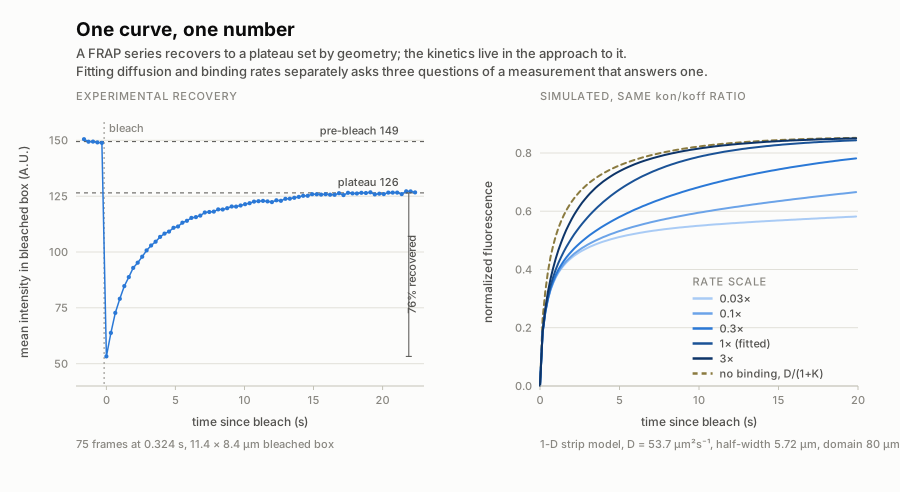
Left: the data I fit, 75 frames at 0.324 s per frame with an 11.4 × 8.4 µm bleached box. The recovery closes only 76% of the gap the bleach opened, because the bleached molecules are gone for good and dilute the pool they return to. Right: why the three-parameter model does not have a unique answer. Every curve holds \(k_{on}/k_{off}\) fixed at the fitted value of 0.60 and only scales the absolute rates; past a certain speed they all collapse onto the same pure-diffusion curve with \(D_{\text{eff}} = D/(1+K)\), and the data can no longer tell them apart.
Model 1: one dimension, because the experiment was designed that way
Fick’s second law is the heat equation, \[\frac{\partial c}{\partial t} = \nabla \cdot (D \nabla c) = D \Delta c,\]
and for the free-diffusion models the binding is hidden inside an effective diffusion constant \(D_{\text{eff}}\) rather than modeled explicitly. The boundary is the nuclear membrane, and no protein crosses it, so the conditions are Neumann: \[\frac{\partial}{\partial t} u = D_{\text{eff}} \Delta u, \quad \frac{\partial u}{\partial \eta}\bigg|_{\partial \Omega} = 0, \quad u(x, 0) = f(x),\]
with \(f(x)\) zero inside the bleached region and \(u_0\) outside.
If you bleach a narrow strip across the nucleus rather than a spot, the problem becomes one-dimensional, and one dimension is where analytical solutions live. Model the nucleus as a rectangle of length \(l\) and the strip as a band of width \(2h\) centered at \(c\). Separation of variables gives modes \(e^{-D\lambda t}(c_1 \sin\sqrt{\lambda}x + c_2\cos\sqrt{\lambda}x)\); the no-flux conditions kill the sines and quantize \(\lambda = (n\pi/l)^2\). What the microscope actually reports is the mean intensity inside the bleached box, so integrate the solution over \([c-h, c+h]\) and normalize by the pre-bleach value \(2hu_0\): \[f_R(t) = \frac{l - 2h}{l} - \frac{l}{h\pi^2}\sum_{n=1}^{\infty} \frac{1}{n^2} e^{-(n\pi/l)^2 D_{\text{eff}} t} \left[\sin\frac{n\pi(c-h)}{l} - \sin\frac{n\pi(c+h)}{l}\right].\]
The first term is the plateau: the bleach removed a fraction \(2h/l\) of the fluorescence permanently, so recovery stops short of 1 by exactly that fraction. In this model the plateau is geometry, not biology—worth remembering, because a genuinely immobile subpopulation would lower it too, and the plateau by itself cannot tell you which you are looking at.
Everything kinetic is in the exponentials, and the slowest mode \(n = 1\) decays over \(l^2/\pi^2 D\), which means the timescale you are fitting is set by the size of the compartment as much as by the protein.
There is a second analytically tractable setup worth mentioning: if you bleach a very small spot in the middle of a large nucleus, the boundary never matters over the timescale of the experiment and you can treat the domain as infinite. Then the Green’s function is a Gaussian, \[G(x, y, t) = \frac{1}{4\pi D t} e^{-x^2/4Dt} e^{-y^2/4Dt},\]
and the solution is a convolution of the initial hole with it. Which idealization is available to you—finite strip or infinite spot—is decided by the microscopist before any math happens.
Numerics
I solved all three models with explicit finite differences: second differences in space with Neumann boundaries, forward Euler in time. The scheme is \(O(\Delta t) + O((\Delta x)^2)\), and being explicit it is only conditionally stable. With \(R = D\Delta t/(\Delta x)^2\), stability needs \(R \leq 1/2\) in 1D and \(R \leq 1/4\) in 2D, so \[\Delta t \leq \frac{(\Delta x)^2}{2D} \quad \text{and} \quad \Delta t \leq \frac{(\Delta x)^2}{4D}.\]
That constraint is more annoying than it looks, because the curve fitter varies \(D\). Every time the optimizer tries a larger diffusion coefficient, the stable timestep shrinks, so the solver has to recheck the CFL number and refine \(\Delta t\) on every function evaluation:
function simulation = f(D, T)
      % Crank down dt until stability is reached
      dt = tStep;
      if D*dt/h^2 >= 0.5
           dt = 0.5*0.5*h^2 / D;
      end

      [f,t] = frapmodel1(L, L/2, w, N, tFinal, dt, D);

      % Interpolate the results back to the experimental time points
      simulation = interp1(t, f, T, 'linear')';
end
The interpolation at the end is the part that makes fitting possible at all. The simulation runs on whatever timestep stability demands—often far finer than the 0.324 s between images—and gets sampled back down onto the experimental time points before the residuals are computed.
The 1D difference operator is the tridiagonal \(B_n\) from Strang, with the corner entries changed from 2 to 1 to impose no flux. The 2D version is the same matrix assembled by Kronecker products, which is the sort of thing that looks like magic the first time and obvious the second:
function [ D ] = diffNeumann2D( N )
% DIFFNEUMANN2D Construct the diff. matrix for 2D diffusion eq. w/no flux
%      Using the 5-point Laplacian molecule

B = diffNeumann1D(N);
M = diag([0.5 ones(1,N-2) 0.5]);
D = kron(M,B) + kron(B,M);

end
Everything is stored sparse, which is what makes it cheap enough to run the solver a few thousand times inside an optimizer.
Fitting is nonlinear least squares (lsqcurvefit). For the single-parameter models I first swept \(D\) over a coarse grid from 10 to 100 µm²/s and started the optimizer from the best point, because starting a local optimizer from an arbitrary guess on a curve-fitting problem is how you end up confidently reporting a local minimum.
Model 2, and then the interesting one
Model 2 is the same thing in two dimensions: nucleus as a square, bleach as a circular spot, and the 5-point Laplacian above. It fits the same data with the same single parameter.
Model 3 is where the physics gets honest. Instead of hiding binding inside \(D_{\text{eff}}\), track two populations—free protein \(u_f\) that diffuses and reacts, bound protein \(u_b\) that only reacts: \[\frac{\partial u_f}{\partial t} = D \frac{\partial^2 u_f}{\partial x^2} - k_{on} u_f + k_{off} u_b, \qquad \frac{\partial u_b}{\partial t} = k_{on} u_f - k_{off} u_b.\]
Now \(D\) is the real diffusion coefficient of the molecule, and the retardation lives in the rate constants where it belongs. The initial condition has to respect the pre-bleach equilibrium: with \(K = k_{on}/k_{off}\) and no flux through the membrane, \(u_f = 1/(1+K)\) and \(u_b = K/(1+K)\) outside the bleached spot, and both are zero inside. Both populations fluoresce, so the observable is \(u_f + u_b\) even though only \(u_f\) moves.
Three fits, and one that isn’t a fit
The 1D model gave \(D_{\text{eff}} = 29.7\) µm²/s. The 2D model gave 31.7 µm²/s, slightly higher with a slightly worse RMSD, but the difference is small enough that I would not read anything into it. The reaction-diffusion model gave \(D = 53.7\) µm²/s with \(k_{on} = 0.187\) and \(k_{off} = 0.310\)—a much larger diffusion coefficient, exactly as it should be, since binding events are no longer being charged to diffusion.
That looked like a success until I swept the parameter space instead of trusting the optimizer. Equally good fits run in a long valley along constant \(k_{on}/k_{off}\). The RMSD surface has no isolated minimum; it has a trench. The optimizer had reported a point on the floor of that trench, and where along it the point landed was decided by my initial guess.
The reason is visible in the numbers. Take the fitted ratio \(K = 0.60\) and compute \[\frac{D}{1+K} = \frac{53.7}{1.60} = 33.5\ \mu\text{m}^2\text{s}^{-1},\]
which is within a few percent of the 31.7 µm²/s that the pure-diffusion model reported. The three-parameter model had quietly reduced itself to the one-parameter model. When binding and unbinding are both fast compared to the time a molecule needs to diffuse across the bleached region, every molecule samples many bound and free episodes on the way in, and the recovery curve only ever sees the time-averaged mobility \(D/(1+K)\). The individual rates leave no fingerprint in the data—that is the collapse in the right-hand panel above.
The models are not wrong, and they are not equally informative. The reaction-diffusion model contains strictly more physics, but the experiment does not contain enough information to identify it. Fitting it to this data is asking three questions of a measurement that answers one. That is not a numerical problem, and no better optimizer fixes it.
What does fix it is more information from outside the curve. You can estimate \(D\) from the molecular weight and the viscosity of the nucleoplasm and hold it fixed. Better, you can mutate the DNA-binding domain, measure the crippled protein with a free-diffusion model to get \(D\) directly, then feed that number into the reaction-diffusion fit and let it solve for the rates alone. Either way the extra parameter has to be pinned by biology, not by least squares.
Further reading
- Axelrod et al., “Mobility measurement by analysis of fluorescence photobleaching recovery kinetics” — the 1976 original
- Sprague and McNally, “FRAP analysis of binding: proper and fitting” — the regimes, and which parameters are identifiable in each
- Carrero et al., “Using FRAP and mathematical modeling to determine the in vivo kinetics of nuclear proteins” — the narrow-strip reduction to 1D
- Beaudouin et al., “Dissecting the contribution of diffusion and interactions to the mobility of nuclear proteins”
- Mueller et al., “FRAP and kinetic modeling in the analysis of nuclear protein dynamics: what do we really know?” — the modeling choices, and how much they matter
- Strang, Computational Science and Engineering — where the \(B_n\) matrices and the Kronecker assembly come from