Building an Optimal Yahtzee Player with Go and Raspberry Pi: Part 1
I didn’t have a Game Boy growing up, but I did have an electronic handheld Yahtzee. It does exactly one thing, and it does it with an admirable lack of distractions.
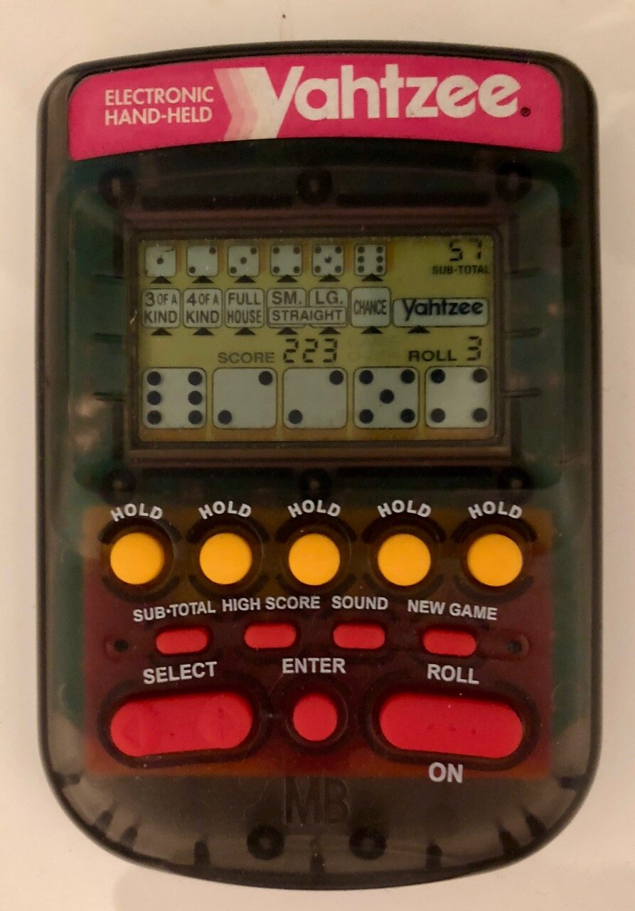
It also keeps an all-time high score. Mine was 407. I got it some time as a child, and it had sat there, unchallenged, through several moves and at least one change of batteries I was genuinely nervous about. Then my girlfriend picked it up, played it for a few minutes casually, and beat it.
I would like to report that I took this well. The mature response is to congratulate her, play a few more games, and reclaim the record honestly. I considered that option, and rejected it.
What I did instead was spend the next several weekends computing the provably optimal strategy for solitaire Yahtzee, and then building a robot to execute it.
In my defense, it’s pretty interesting! When is a zero worth taking to preserve a better category for later? And, since the goal is not a good average score but specifically to beat one particular number, how does the strategy change versus a naive expected value maximization? When should a player abandon an unpromising game and start another?
This is the first of three posts about answering those questions. Here I will turn solitaire Yahtzee into a dynamic-programming problem. In Part 2, I will show the Go implementation that computes the strategy tables; Part 3 puts the strategy in control of the physical game.
The rules
In solitaire Yahtzee, a turn starts with five dice. You may keep any subset and re-roll the rest up to twice, then score the resulting five dice in one of thirteen categories. Each category can be used only once.
The familiar categories—three of a kind, full house, straights, chance, and Yahtzee—make the immediate choice interesting. The constraints make the whole game interesting. The upper section awards a 35-point bonus at 63 points, and a second Yahtzee can trigger a 100-point bonus plus the joker rules. A pair of sixes is not just a pair of sixes: it might be progress toward the upper bonus, a chance score, a future Yahtzee, or the only thing preventing an ugly zero.
For perspective, the best expected score under the standard solitaire rules is about 254.589 points (Pawlewicz). A score of 407 is well above average!
A state is more than the dice
The dice alone do not determine an optimal move. The decision also depends on:
- which scoring categories are already filled;
- the upper-section subtotal, up to the 63-point bonus threshold;
- whether a Yahtzee bonus is still possible; and
- where the player is within the current turn.
For maximizing expected value, one need not consider the current total score. Every future point is worth one more point, so two games with the same open categories and bonus status have identical future decisions even if one happens to be ahead.
Solve it from the end backwards
Let the value of a game state be the best expected number of points still available from that state. At the end of a completed game, that value is zero: there are no future points left to earn. On the final roll of a turn, the value is simply the best available scoring box:
value(final roll) = max over open boxes of
    points scored now + value(next game state)
Before the final roll, each possible set of held dice has an expected value over the re-rolls that follow. The player chooses the hold with the largest expected value. Before the first roll, the same idea averages over every possible initial roll.
Stated more formally, solitaire Yahtzee is a finite-horizon Markov decision process. The state \(s\) is the score-sheet summary above; the actions are the choice of which dice to hold and, at the end of a turn, which category to fill; the transitions are the dice, which are the environment’s move rather than the player’s; and the reward is the points written down. Because the horizon is fixed at thirteen turns and every point counts equally, there is no discount factor. Solving the game means computing the optimal value function \(V^*(s)\), the expected points still to be earned from \(s\) under optimal play, which satisfies a Bellman optimality equation. Writing \(U_k(s, r)\) for the value of holding roll \(r\) with \(k\) re-rolls left in the turn, \[\begin{aligned} U_0(s, r) &= \max_{c \,\in\, \mathrm{open}(s)} \Big[\, \mathrm{points}(c, r) + V^*(s \oplus c) \,\Big], \\ U_k(s, r) &= \max_{h \subseteq r} \; \mathbb{E}_{r'}\big[\, U_{k-1}(s,\, h \cup r') \,\big], \qquad k = 1, 2, \\ V^*(s) &= \mathbb{E}_{r}\big[\, U_2(s, r) \,\big], \end{aligned}\]
where \(s \oplus c\) is the state with category \(c\) filled. The alternation of maximization over the player’s choices with expectation over the dice is expectimax: decision nodes take a max, chance nodes take a probability-weighted average. There is no minimizing opponent, which is what makes solitaire Yahtzee tractable in a way that adversarial games are not.
This recurrence can be solved with dynamic programming because it has both optimal substructure, since an optimal strategy from \(s\) contains optimal strategies for every successor state, and overlapping subproblems, since a huge number of distinct play sequences arrive at the same score sheet. Rather than recompute those subtrees, the solver tabulates each \(V^*(s)\) exactly once.
Because every turn permanently consumes a category, the state graph is a directed acyclic graph, and filled-box count is a topological order on it. So the table is filled in reverse—score sheets with twelve filled boxes first, then eleven, and so on down to the empty sheet—and every transition on the right-hand side refers to a state whose value is already final. One backward sweep suffices; no iteration to convergence is required, because there are no cycles for value to propagate around. This is backward induction, and the game-playing literature calls the exhaustive tabulated form retrograde analysis, the same technique used to build endgame tablebases in chess and checkers.
The approach is well established for Yahtzee; Woodward, Glenn, and others provide excellent treatments. I wanted to make the calculation concrete enough to drive a real device.
Dice symmetry pays for itself
There are \(6^5 = 7,776\) ordered five-die rolls, but the order of dice on the screen does not affect the strategy. A roll containing two ones, one two, one four, and one six is the same multiset no matter which physical position shows each die. There are only \(\binom{5 + 6 - 1}{5} = 252\) such multisets.
They are not equally likely: a Yahtzee has one ordering, while five different values have 120. The solver evaluates only the 252 distinct rolls and weights each by its multinomial probability. It similarly treats equivalent holds as one choice. That reduction makes exhaustive evaluation practical without changing the result.
Different goals produce different strategies
Maximizing expected score is only one reasonable objective. If the goal is to beat a specific high score \(S\), the useful question becomes: which move maximizes the probability that the final score is at least \(S\)?
Instead of storing one expected value at each state, the solver can store the whole tail distribution of possible remaining scores. At decision time it reads the entry for the score still needed. This produces a riskier policy: when the goal is 407, taking a safe small score can be worse than chasing the unlikely outcome that keeps 407 possible.
Restarting is an action too
Optimizing the chance of success in a single game still assumes that every game must be finished. A physical player has another action: press New Game! Once a run is so far behind that it has little chance of reaching the target, finishing its remaining turns consumes time that could be spent on a fresh run.
I modeled this as a stochastic shortest-path problem. Define the cost of a state as the expected number of future rolls until a target score is achieved. A game that has reached the target costs nothing more — it is over, since the boxes still open could only add points; a game that runs out of boxes short of the target costs the price of beginning again; and every roll adds one unit of work. Continuing is useful only when its expected cost is lower than restarting immediately.
This is much harder to solve because it’s circular: the value of a failed terminal game depends on the expected cost of a new game, which is itself what we are solving for. The obvious fix is to feed the answer back: guess the cost of a fresh game, run the ordinary backwards calculation, take the new value it gives the opening position as the next guess, and repeat until it settles.
That works, but barely. Writing \(g\) for the guess, a pass hands back \[f(g) = W + (1 - p_0)\,g,\]
one game’s worth of real work \(W\), plus the guess over again on the \(1 - p_0\) of the time that game fails. The map is a contraction, but its slope is \(1 - p_0\), so each pass removes only a \(p_0\) fraction of the error — and \(p_0\), the chance of beating the target in one game, is the small number that made the problem interesting in the first place. For a target of 407 it is about 4%, so settling would take hundreds of passes over a hundred million states.
A budget for giving up
The solver answers this state by state, but a stripped-down version of the same question has a closed-form answer — one that explains the shape of the policy, and rescues the convergence above.
Suppose a game lasts \(N\) turns, each turn costs \(T\) units of work, and \(p_k\) is the probability of eventually beating the target given the position after \(k\) turns. A complete game therefore costs \(TN\) and succeeds with probability \(p_0\).
Let \(E_0\) be the expected work to beat the target starting from a fresh game. One game costs \(TN\) to play, and with probability \(1 - p_0\) it fails and leaves us exactly where we began: \[E_0 = TN + (1 - p_0)E_0 = \sum_{k=0}^{\infty}(1-p_0)^k \, TN = \frac{TN}{p_0}.\]
From a position \(k\) turns in, finishing costs \(T(N-k)\), and with probability \(1 - p_k\) that work buys nothing and we start over: \[E_k = T(N-k) + (1 - p_k)E_0.\]
Continuing is worth it exactly when \(E_k < E_0\), and the \(T\)s and \(N\)s oblige by cancelling: \[T(N-k) + (1-p_k)\frac{TN}{p_0} < \frac{TN}{p_0} \quad\Longleftrightarrow\quad p_k > p_0\left(1 - \frac{k}{N}\right).\]
The budget is linear. A game is worth continuing as long as its chance of success has fallen by less than \(p_0/N\) per turn on average, and the allowance is the same in every turn.
That derivation also repairs the convergence problem, because it prices a policy in closed form instead of one attempt at a time.
Look again at what a pass produces. It ends holding a policy, and the number it returns, \(f(g) = W + (1-p)g\), is what a single attempt of that policy costs when failure is charged the current guess. But the algebra above prices the same policy with no guess in it at all: run it until it finally succeeds and it costs \(W/p\). The gap between the two is precisely the geometric series that the naive iteration was going to accumulate a few percent at a time over the next several hundred passes.
That ratio cannot be recovered from an ordinary value function, because the guess has already been folded into every number in it. So feed back the ratio instead of the value: each state stores the two quantities its cost is built from — the rolls this game still expects to take, and the probability that it beats the target — carried along by the same backward pass, at essentially the same cost per pass. When the pass ends, \(W\) and \(p\) for the policy it just found are sitting separately at the opening position, and \(W/p\) is what that policy actually costs, in the \(TN/p_0\) form derived above. Use it as the next guess.
That update is Newton’s method. Since \(f\) is a minimum over policies of functions affine in \(g\), it is concave and increasing with slope \(1-p\), and the Newton step for the root of \(f(g) - g\) is \[g - \frac{f(g) - g}{f'(g) - 1} = g - \frac{W + (1-p)g - g}{-p} = \frac{W}{p},\]
the ratio update exactly. (Repeatedly minimizing a ratio by solving the linearized problem it induces is Dinkelbach’s algorithm; in the language of dynamic programming, feeding back \(W/p\) turns value iteration into policy iteration.) Concavity keeps every tangent line above \(f\), so the iterates stay above the answer and descend to it — from above, quadratically, and in practice stopping outright once the policy quits changing. A handful of passes rather than hundreds, for the price of storing a numerator and a denominator instead of their quotient.
What this policy looks like in practice is … amusing. When the target is a score as high as 407, \(p_0\) is very small, and the linear budget is correspondingly stingy: the strategy needs the game in front of it to stay on a near-perfect trajectory. One mediocre opening turn is usually enough. The optimal high-score player therefore spends the overwhelming majority of its existence taking a single look at a fresh game and immediately restarting, like someone speed-dating who has decided within four seconds that this is not going to work out.
It is correct — the cheapest way to find a very good game is to sample many games rather than to nurse a bad one — but it does mean that a strategy optimized to beat a high score plays visibly worse Yahtzee than one optimized for expected score, and looks impatient doing it. It also has an unfortunate implication for anyone planning to execute this policy by hand on a physical device, which we will come to in Part 3.
What remains to compute
The score-independent formulation in my implementation has 536,448 reachable game states. It is large enough to reward careful code, but small enough to solve exactly on a normal computer. Tracking the running total for the restart policy expands the reachable space to 111,636,963 states, so that version needs more memory discipline and evaluates one target score at a time.
The next post is about those engineering choices: compact game and roll representations, reusable turn calculations, and strategy tables that a web service—and eventually a Raspberry Pi—can query quickly.
Further reading
- Phil Woodward, “Yahtzee®: The Solution”, Chance 16(1), 2003.
- James R. Glenn, “Computer Strategies for Solitaire Yahtzee”, 2007.
- C. J. F. Cremers, “How to beat high scores in Yahtzee”, master’s thesis, 2002.
- Jakub Pawlewicz, “Nearly Optimal Computer Play in Multi-player Yahtzee”, 2010.